20.8 Probability distributions
The risk associated with alternatives under consideration can be displayed graphically, using a probability distribution histogram, or risk profile. A probability distribution histogram graphs the values (i.e., payoffs) and path probabilities of all terminal nodes within a strategy. This is for models with a single payoff.
This analysis is deterministic (no randomness) and simulation generates probability distribution graphs based on long runs of stochastic, random walks.
Open the Oil tutorial example model, Oil Drilling Problem.trex. This model has some interesting elements, including multiple decisions nodes. The figure below os the strategy "No Soundings".

To create your first probability distributions using TreeAge Pro, start by analyzing a chance node.
To view a probability distribution histogram:
-
Select a chance node – in this case the topmost chance node labeled Drill for Oil, in the No Soundings section of the tree.
-
Choose Analysis > Probability Distribution.
-
Use the default Histogram Type: Probability Distribution.
-
Use the default Histogram Parameters. Select OK.
TreeAge Pro displays the analysis results in a graph window as shown below.
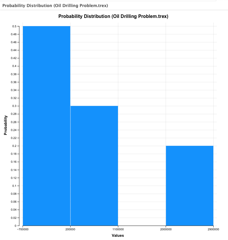
There are different options available to customize the Histogram using the links on the right hand side.
More details about customizing histograms can be found in Graphs - Customizing Histograms section.
20.8.1 Probability Distribution Secondary Reports
Every graph window includes a set of "Actions" and other settings to the right of the graph. The Probability Distribution graph includes two links at the top.
-
Text Report (Bars): Show the numerical source data for the graph. This changes as we change the number of bars.
-
Text Report (Raw): Show the numerical source data in detail including the node, path probability and node EV.
In the example Probability Distribution graph (not the CDF), TreeAge Pro displays a separate bar for each possible payoff. However, this will not always be the case, as some outcomes with similar values may be merged into a single bar within the graph.
Initially, the value range is divided into a reasonable number of intervals. The height (i.e., probability) of a bar is the sum of the path probabilities of all terminal nodes with payoffs in that interval. The height of all bars sums to 1.0 (100%). The vertical axis will scale to the height of the highest bar.
The value/probability associated with each bar can be accessed via the graph's Text Report (Bars).

The Text Report (Raw) is similar, except that it will include every outcome (with no summarization by bar) along with the node name associated with the outcome.

20.8.2 Downstream decision nodes
As noted above, the Oil tutorial example model, Oil Drilling Problem, includes multiple decisions. To see how the probability distribution analysis is affected by downstream decision nodes, analyze the Seismic Soundings chance node. Each of this node’s branches is a decision node. See below.
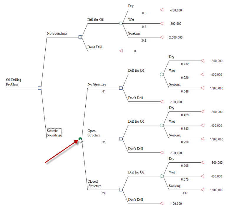
If there are decision nodes anywhere to the right of the analyzed node, as in this analysis, TreeAge Pro calculates expected values, and then selects an optimal strategy at each downstream, or deferred, decision. The histogram only includes terminal nodes from the optimal path, therefore the path probabilities in the histogram will still sum to 1.0. To see which terminal nodes are in the optimal path, you can roll back the tree.
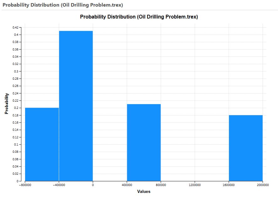
The information which is presented in the Probability Distribution is to allow the modeller to make decisions based on the range of possible outcomes/valuse and the likelihood of these outcomes happening. Using the PDF dialog on the right-hand side of the graph, changing the number of intervals or intervals size can assist in this process. There are links to the two Text Report links to the right of the graph to generate reports showing the underlying data and will give you information about which outcomes are most likely.
The Text report (Bars) displays the individual bar values and their probabilities.
The Text report (Raw) shows the individual terminal nodes that contribute to each bar.
20.8.3 Cumulative Probability Distribution
If the option "Cumulative Probability Distribution" is selected from the same node, a different graph is presented.
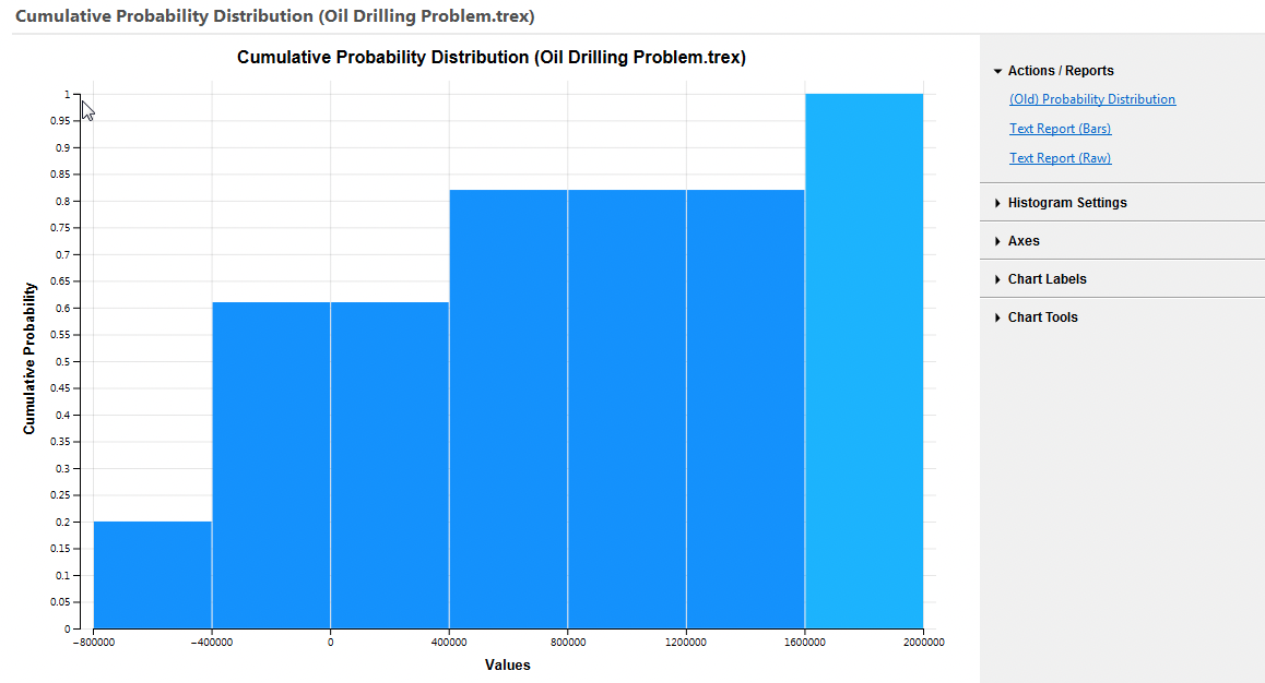
This graph shows a complete EV range for all outcomes in the model along with the cumulative probability that the outcome will be less than or equal to a specific bar in the range. In this model there is a 50% chance that the EV will be less than or equal to approximately -600,000, while there is an 80% chance that the EV will be less than or equal to approximately 500,000. Greater precision is available via the secondary reports, which are described later in this section.
20.8.4 Comparative probability distributions
Multiple, cumulative probability distributions can be displayed in a single graph, allowing graphical comparison of options. In a comparative distributions graph, the cumulative distributions are displayed in outline, instead of using filled bars. This format enables graphical comparison of strategies based on their risk profile.
Details about the graphical interpretation of comparative probability distributions are provided later in this chapter, in the section on dominance.
When a single decision node is selected, the Analysis menu displays the Comparative Distributions command. The comparative distributions analysis can be tried at the root decision node in the Oil Drilling Problem tree.
To generate a comparative probability distribution graph:
-
Select a decision node.
-
Choose Analysis > Comparative Distributions from the menu.
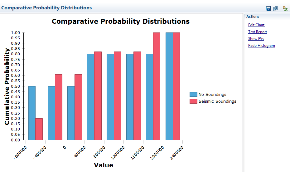
The resulting graph displays the outlines of the cumulative probability distributions for the competing options Seismic Soundings and No Soundings. The outline for a strategy is marked at each corner (where the cumulative probability “curve” rises) with that strategy’s symbol, as listed in the legend to the right of the graph.
20.8.5 Dominance in probability distributions
Comparative probability distributions can be interpreted graphically, by evaluating conditions of dominance. There are two types of dominance that can be identified relatively easily: deterministic and stochastic (also called absolute and extended dominance). Conditions of dominance can provide more insight into a decision than simple expected value comparison.
Deterministic dominance occurs when one option not only has the best expected value, but its worst possible outcome is better than (or equal to) the best outcome of any other option. It can be identified as follows:
-
if optimization requires maximizing value (e.g., profit), the worst “bar” of the dominant option (its left-most vertical line) lies on, or to the right of, the best (right-most) “bar” of the dominated option(s);
-
if optimization requires minimizing value (e.g., costs), the worst “bar” of the dominant option (its right-most vertical line) lies on, or to the left of, the best (left-most) “bar” of the dominated option(s).
The kinds of problems in which decision analysis is applied will not often display deterministic dominance, however. Stochastic dominance is more likely. Conditions of stochastic dominance — also called extended or probabilistic dominance — are identified as follows:
-
if optimization requires maximizing value, the entire outline describing the stochastically dominant option lies to the right of the dominated option’s outline — the lines can touch for part of the graph, but never cross;
-
if optimization requires minimizing value, the outline describing the stochastically dominant option lies on, or to the left of, the dominated option’s outline.
20.8.6 Combining probability distribution graphs
Two probability distribution graphs can be combined to generate a single graph demonstrating the full range of value outcomes from both models/strategies. This could be used to assess the financial risk from two separate legal cases.
WARNING! The “combined” probability distribution — representing the overall risk from two or more cases being litigated (or arbitrated) — is only valid if the cases being combined are completely independent of each other.*
That means that, when the outcomes of two cases (for example) are being combined, the Case #2 tree — its structure and every one of its probability and award assessments — would be completely unaffected by the outcome of Case #1; i.e., that none of the issues or assessments making up Tree #2 would vary regardless of which path the trier were to follow in the Case #1 tree.
This condition would not be met when the matters being combined involve similar claims/facts/witnesses, and knowing how the trier reacted to the claims/facts/witnesses in a first case would influence your odds of success in a later trial or arbitration. [Note, however, that even in this situation it is usually still valid to combine the Expected Values of the related matters.]
One situation where the condition of complete independence could be met, and where a combined probability distribution could be useful to a business client, would be where the client is a party to two (or more) significant but completely unrelated lawsuits, and for business planning purposes wants to understand the overall probability of ending up with various overall results from these significant litigations/arbitrations.
Here we will combine the probability distribution graphs from the Litigate strategies of two Legal Example Models - BreachOfContract.trex and Legal-Negligence.trex shown below.


Combining the two independent graphs will combine every model scenario from the first case with every model scenario from the second case. Let's look at the highest value outcomes for each case as an example.
-
In Case 1 above, the highest value is $4M with a likelihood of 6%.
-
In Case 2 above, the highest value is $4.4M with a likelihood of 12%.
-
The combined highest value of both cases is...
-
Value is the sum of the two values: $8.4M.
-
Likelihood is the product of the two probabilities: 0.7%
-
In this way, all the combined possible outcomes are generated - summing the values and multiplying the probabilities.
The resulting combined graph is shown below.

Note the furthest bar to the right is $8.4M and 0.7% likely.
The Text Report (Raw) link shows the individual scenario combinations that are bundled into bars in the graph. The bottom portion of that report is shown below. Note the last row is the highest value combined scenario described above.

