26. Bayes Revision
If your model includes imperfect tests or forecasts followed by decisions, you may wish to utilize TreeAge Pro’s Bayes’ revision feature.
TreeAge Pro can automatically perform probability revisions using Bayes’ theorem. The process occurs once during the initial construction of the model. Based on your answers to a few questions, TreeAge Pro will generate a set of variable definitions that calculate the revised probabilities. The probability expressions will be recalculated every time the model is evaluated and results can change as your estimates of prior and likelihood probabilities (see below for definition) change.
Bayes’ revision is implemented in the tree editor window. Bayes’ revision in the tree window is able to revise probabilities automatically based upon a single test. The process can be performed more than once within a model for different tests.
There are two methods of applying Bayes' theorem on your model, each of which is described later in this section:
Probability revision using Bayes' theorem
Bayes’ revision allows decision makers to calculate decision probabilities from likelihood probabilities. Likelihood probabilities, or forecast likelihoods, are answers to questions such as, “If this test is performed on a part known to be faulty, what is the probability of a positive result indicating a problem?” This type of probabilistic information is often available, but is not immediately useful in making decisions. What's needed are the decision probabilities, which address questions such as, “If a particular part tests positive, what is the probability that it is really faulty?”
The decision probabilities are so named because, in the real world, they are the probabilities upon which decisions are based. These are also sometimes called posterior (or a posteriori) probabilities.
The basic formula for revising probabilities is:
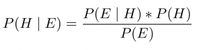
where H is the hypothesis (e.g., faulty or not faulty) and E is the evidence (e.g., test result). The formula is applied once for each hypothesis-evidence combination — for example, P(not faulty positive), or the probability not faulty given a positive test result. P(H) represents the prior (or a priori) probability of the condition. P(E) is a marginal probability, calculated as part of the revision.
A simple numeric illustration
The following example is designed to offer a sense of the potential usefulness of Bayes’ revision. If you are already familiar with the types of applications that require Bayes’ revision, you may want to skip this section.
Consider an automated test for a defect in a semiconductor. The defect is present in 1% of the items under scrutiny. It has been demonstrated that the available test will detect 98% of the faulty materials, meaning that 2% of those pieces with the defect will not be picked up by the test. Also, the test is known to incorrectly identify as faulty 3% of those pieces that are without defect.
You have considered installing a machine to perform this test in your facility. What is the likelihood that a part which tests positive actually has the defect? How certain can you be of parts that tested negative don’t have a defect? The information about the accuracy of the testing equipment provided above does not directly answer these crucial questions.
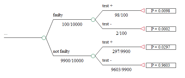
Let’s say we have a batch of 10,000 items to be tested.
If the estimated prior probability of defect is 1%, we would expect 100 items in the batch to have the defect. Of these, about 98 should test positive. Of the 9,900 pieces without the defect, we said approximately 3% (297) would test positive.
Thus, a total of 395 (297 + 98) test subjects would test positive (this is one of the marginal test probability).
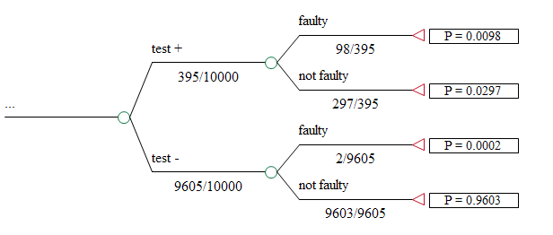
The Bayes’ revision formula is intuitive when illustrated and worked out using a tree, as shown below.
The first revised decision probability is the ratio 98/395, or approximately 25%. This is the probability that a positive test actually indicates the presence of the defect. In this case, 75% of the positive tests are in error. The other decision probabilities are similarly calculated. With this information, a decision maker could compare the performance of the new test with existing methods or competing technologies.