Using Debug functions to control output

30.2 Using Debug functions to control output

Most of the time, you will use Tree Preferences to control the debug info written to the Calculation Trace Console. However, you can also generate debug info by placing debugging functions directly in the model.

The following table lists the specialized commands which can be executed to debug a model.

Important note: All of these commands have zero ("0") value and can be added to expressions without changing the value of the expression.

Function syntax	Description
DebugOn() previously Debug("1")	Turn the calculation trace setting on. After issuing this command, all internal calculations will be written to the Calculation Trace Console.
DebugOff() previously Debug("0")	Turn the calculation trace setting off. After issuing this command, internal calculations are no longer written to the Calculation Trace Console.
DebugExport(filename)	Export the current contents of the calculation trace console to a .txt file to a specific location with a specific name. An example of what we could replace file with is: filename = path + "name_of_file" + Str(_trial) + ".txt" where path = "X:\\Testing\\DocModels\\Output_files\\"; name_of_file = the new name of the file where we save the export; Str(_trial) = the number of the current _trial in the model; and .txt = sets the file type.
DebugExport(index)	Export the current contents of the calculation trace console to a file with the same name as the model, followed by "_trace_" plus the index and with the file extension .txt. The .txt file will be located in the same folder as the original model.
DebugClear()	Clear all the output in the calculation trace console.
DebugWrite(text)	Send the text argument to the console with a blank line before and after it. Note the text will only be written if debugging is turned on via the Tree Preferences (All or Selected) or via the DebugOn() function.
DebugWriteForce(text)	Send the text argument to the console with a blank line before and after it. Note the text is written regardless of whether debug output is turned on or off.
DebugTime()	Write the current date/time including milliseconds to the console. Note the text will only be written if debugging is turned on via the Tree Preferences or via the DebugOn() function.
DebugTimeForce(text)	Write the current date/time including milliseconds to the console. Note the text is written regardless of whether debug output is turned on or off.

If the Debug() function requires the debug output to be turned on then this can be done either via turning on 'Show Output for All' in the Tree Preferences or by using the DebugOn() function.

The Debug() functions can be useful when combined with some of the keywords which are specifically used to select individual trials in Monte Carlo analysis. More information about these keywords can be found on the section about Customizing Simulations, specifically in the section about Monte Carlo special variables. The Model Debugging and Validation Chapter has examples using a number of the Debug tools to debug models.

Below are a couple of examples using the Debug() function.

30.2.1 Example: Using the calculation trace dynamically

It is often useful to turn the Calculation Trace on to examine specific calculations and why the model might be failing. For models with a large number of calculations, it is prohibitive to turn the Calculation Trace on for all trials (microsimulation) and samples (sensitivity analysis). It may take too long for the Calculation Trace to get to the point where the model is failing.

In these situations, looking at the internal calculations from the Calculation Trace Console for all trials may not be required but you may want to look at a specific trial's values.

To pinpoint a specific trial's calculations

Examine the Special Features example model, Debug MicrosimulationCancerModel.trex.

Consider an error which is occurring for trial 999 in a Monte Carlo simulation. To look at the internal calculations for just trial 999, the model has the following definitions included:

Create a special simulation variable to turn on the calculation trace before trial 999 goes through the model: _monte_pre_trial_eval = if(_trial=999; DebugOn(); 0).
The special variable/keyword _monte_pre_trial_eval is a built in keyword in TreeAge Pro. It will ensure the expression it equals will be evaluated before every trial in the model is evaluated. In this case the expression will turn the debug function on, using DebugOn(), if _trial = 999. Otherwise the expression will do nothing.
Create a special simulation variable to turn off the calculation trace after trial 999 has finished with the model: _monte_post_trial_eval = if(_trial=999; DebugOff(); 0).
The special variable/keyword _monte_post_trial_eval is a built in keyword in TreeAge Pro. It will ensure the expression it equals will be evaluated after every trial in the model is evaluated. In this case the expression will turn the debug function off, using DebugOff(), if _trial = 999. Otherwise the expression will do nothing.

Running microsimulation on the model with 2,000 trials will show one output in the Calculation Trace Console, that is the calculations for _trial = 999.

Other useful keywords, like _monte_pre_trial_eval, can be used to customize your models. They can be found in the section about Customizing simulations.

30.2.2 Example: Locating distribution sampling errors

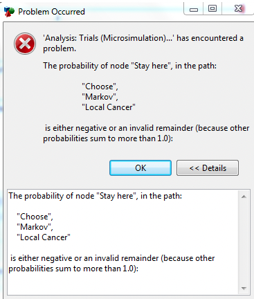
A common Analysis Error which occurs is related to distributions. Distributions may be defined appropriately when sampled independently. However, a combination of distribution samples can cause probability errors during analyses. A typical Error message is shown in the figure below, which was generated by running Probabilistic Sensitivity Analysis on the Special Features example model, Debug WriteForce MarkovCancer.trex.

Open the example model, Debug WriteForce MarkovCancer.trex and examine the two distributions.

Both Dist_p_Local_Death and Dist_p_Local_Mets are Beta distributions with the same parameters, mean of 0.4 and standard deviation of 0.1.

Both the distributions are sampled per Expected Value, so when we run Probabilistic Sensitivity Analysis every re-calculation of the model will re-sample from the distributions.

In the Tree Preferences we have chosen to turn on seeding and threading. We have turned seeding on to replicate the same results over and over again. This is a useful technique if you are trying to locate a problem in a model which keeps moving when the random number seed changes. We have chosen to run the model with a single ("1") thread which means that the calculations have to take place in order. You can find out more about these options in the Tree Preferences section.

Run the model by selecting the decision node and then Analysis > Probabilistic Sensitivity Analysis. Run 100 samples. The error message should be similar to the Figure above.

To debug this model we have created a variable which we can add to any variable in the model to examine specific output. The variable is:

outputDebug = DebugWriteForce("Sample= " + str(_sample) + ", Prob LocToMets=" + str(Dist_p_Local_Mets) + ", Prob LocToDead=" + str(Dist_p_Local_Death))

Consider the the first few elements of the variable ouputDebug:

DebugWriteForce( text here ) : This is the command which instructs the model to write what ever is in the place of "text here" to the Console. This command will work even if debug is turned off in the Tree Preferences.
"Sample = " + str(_sample) : This is some of the text which is included within the executable section of the function DebugWriteForce. It has three elements:
- Quotation marks: Anything written within " " will be written to the colsole. In this case "Sample = ".
- The ' + ': This is used to concatenate expressions. In this case, "Sample = " will be first followed by the interpretation of str(_sample).
- str(_sample): The function str() converts whatever is in the brackets to text for the screen. This example converts the keyword _sample (which gets the current sample number) to a string. We would expect in Probabilistic Sensitivity Analaysis (PSA) a new sample number for each of the PSA samples.

The other elements which make up the variable are similar. Instead of the sample number being written to the screen, the value of Dist_p_Local_Mets and the Dist_p_Local_Death are written respectively.

This variable outputDebug can be added anywhere within the model. Because all the debug functions have zero value adding this variable to another variable in the model has no impact on the value calculated. In the example model you will see we have added the variable to the probability under the branch at Local Cancer > Progress to Metastases. The figure below shows the output in the Calculation Console Trace immediately before the Error happens.

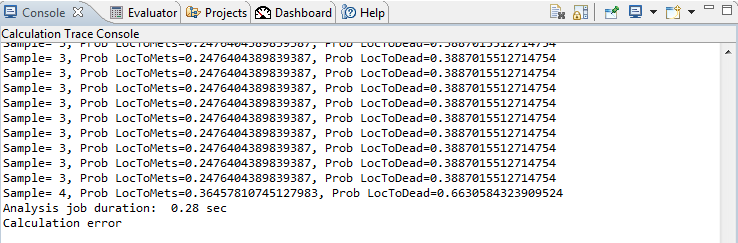
The error can now be identified in the model. The sum of all the probabilities at the Local Cancer node must be 1. By including the '#' under the Stay Here branch, the model first calculates the probabilities at the other two branches and the calculates the probability at the Stay Here branch. The output above shows that when the PSA gets to the forth sample, the values which are generated from the Beta distributions from pLocalToMets = 0.365 and from pLocalToDeath = 0.663. The sum of these alone is greater than 1 so the model is unable to define the probability under the Stay Here branch. Whilst both the distributions are valid, the Example model needs to reconsider their combined probabilities.

In addition, look at the String Processing section for syntax related to creating string expressions for the DebugWrite and DebugWriteForce functions.