35.7 Using non-coherent probabilities/Normalization
TreeAge Pro normally requires the branch probabilities of each chance node to sum to 100%. Probabilities that meet this requirement are referred to as “coherent.” However, there are some situations where it may be useful to relax or remove this restriction (i.e., dynamic cohort analysis, parallel trials).
TreeAge Pro provides options to override the normal chance node functionality - either for the entire tree or for a specific chance node.
You are urged to employ these options cautiously after giving careful consideration to the potential hazards of overriding normal chance node functionality. Do not use this option simply because your probabilities are not summing to 100%. This is usually an error condition caused by probability expressions and/or distribution samples. Such an error must be corrected to generate valid analysis output.
35.7.1 Allowing non-coherent probabilities at a specific node
You can allow non-coherent probabilities at specific chance and Markov nodes in the model; other node types do not allow this option. It is best to allow non-coherent probababilities only at specific nodes rather than for the whole model as described in the next section.
To change the probability coherence option for a node via the context menu:
-
Right-click on a chance node or a Markov node.
-
Within the context menu, choose Change Coherence > your desired option.
To change the probability coherence option for a node via the main menu:
-
Select a chance node or a Markov node.
-
Choose Node > Probability Coherence > your desired option.
The coherence options available are:
-
Use Tree Preference setting: Do not override for this node. Use the option from tree preferences.
-
Allow < > 100% for this node: Allow non-coherent probabilities at this node.
-
Do not allow < > 100% for this node: Do not allow non-coherent probabilities at this node.
-
Normalize probabilities: Normalize probabilities to force them to sum to 100%.
If the probabilities are allowed to be non-coherent, you will get odd expected values. This is not recommended, except when you need to add/subtract from the cohort size (dynamic cohort modeling).
Normalization will take the probabilities that do not sum to 100% and normalize them to make them sum to 100%. For example, if you had probabilities 0.3, 0.4 and 0.5, the total sum would be 1.2. By dividing each probability by 1.2, the probabilities would be normalized.
Note that you can use probability normalization along with the complement probability hashtag. If you have three branches - two probability expressions and the hashtag, normalization will only occur if the two expressions sum to more than 100%. In that case, those probabilities will be normalized and the hashtag will calculate to 0.
|
Original |
Normalized |
|
|---|---|---|
|
Prob1 |
0.3 |
0.25 |
|
Prob2 |
0.4 |
0.333333 |
|
Prob3 |
0.5 |
0.416667 |
|
Sum |
1.2 |
1.0 |
The Special Features tutorial example model ProbabilityNormalization demonstrates this technique.
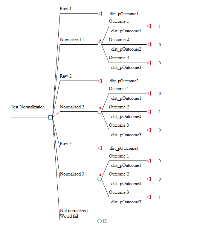
The first 6 strategies alternate between probabilities sampled from a distribution and the normalized probabilities. The Raw 1 strategy simply reports the first probability sampled from a distribution. The Normalized 1 strategy returns the probability after it has been normalized at the chance node.
The bottom strategy is excluded from the analysis because it would fail since the probabilities are not normalized.
Note the red flags above the nodes with probability coherence overrides. This indicator helps identify when a node will function differently from the rest of the model. Node branch comments are automatically created with the text "(Node Probability Override)", which in turn causes the flags to be presented.
Run Monte Carlo Simulation/Sampling on the model to see the original and normalized probabilities. The summary mean values below illustrate the normalization.
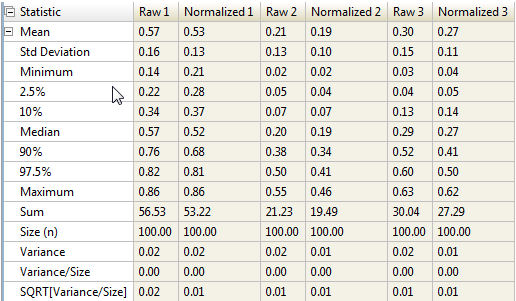
Note that the original mean value for probabilities 1, 2 and 3 are 0.57, 0.21 and 0.30, while the normalized mean values are 0.53, 0.19 and 0.27.
Contrast this with results from the Special Features tutorial example model ProbabilityNonCoherence. In that model, no normalization is done; the bad probabilities are simply allowed. This is not recommended.
35.7.2 Allowing non-coherent probabilities for the entire model
A Tree Preferences option allows non-coherent probabilities for the entire model. However, it is recommended that non-coherent probabilities be allowed at specific nodes instead. See next section.
To disable errors when using non-coherent probabilities:
-
Choose Tree > Tree Preferences from the menu or click F11 to open the Tree Preferences Dialog.
-
Navigate to the preference category Calculation > Other Calculation Settings.
-
Check the option "Allow probabilities to not sum to 100%".
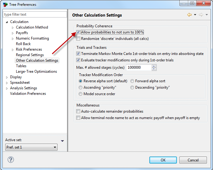
As precautions against unintended use, the status bar at the bottom of the TreeAge Pro window displays text to notify you that this setting is active.

Non-coherent probabilities are not compatible with microsimulation (first-order trials) unless integer values are used for the probabilities for parallel trials, but can be used in probabilistic sensitivity analysis using expected value calculations.
35.7.3 Reporting future net present values in the tree
Discounting is normally used to generate the net present value of future values. In nearly all cases, the net present value of future values is less than the future value itself due to inflation. Decision analysis is then performed using the net present values for all values in the model.
If a decision is to be made at an intermediate node in the tree which occurs in the future (e.g., options valuation), it may be necessary to calculate the net value at the time of the future decision rather than the present time. This would require discounting from the distant future value back to the less distant decision point rather than back to the present.
In situations where it is appropriate, it is possible to use non-coherent probabilities to perform the discounting instead of discounting each terminal node payoff. Net present value discounting is generally performed by dividing by (1+discount_rate)^time. By turning off probability error checking, this division could instead be performed on each branch probability. If done correctly, the expected values calculated at the root node of the tree will be unchanged from a standard, payoff discounting model. See the TreeAge web site for more information.
As with other uses of probability non-coherence, care must be taken to ensure that hidden probability errors are not unknowingly introduced.
35.7.4 Discrete and dynamically-sized Markov cohorts
Normally, decision trees are used to calculate an expected, or average, value. In budget-oriented or population-based modeling, however, the ultimate goal may be to determine not an average, but an overall cost or benefit. In some cases, this can be accomplished simply by multiplying the expected value by some number (e.g., the number of projects, or the size of a population). If TreeAge Pro’s probability coherence requirement is turned off, an equivalent option would be to do the multiplication via tree “probabilities.”
Non-coherent probabilities might be used to model a population whose size changes over time. For example, in a Markov model built using the Healthcare module, the starting population can be initialized — sized and distributed among possible health states — prior to the Markov calculation. Then, during Markov calculations, non-coherent probabilities could be used to change the size of the population, modeling entry from other populations (i.e., from uninfected to infected) or internal population growth (births). For an example of this technique, please refer to the Dynamic Cohort Models Chapter.
When allowing non-coherent probabilities, a sub-option to randomize “discrete” individuals is available that will maintain integer probabilities at subsequent chance nodes — in effect, keeping individuals whole by randomizing them at chance nodes (during any analysis, not just simulation). This might be relevant, for example, where small probability events are critical (i.e., in a vaccination model where continued transmission of a contagious disease requires a “whole” carrier).