44.7 Appendix: Goodness of Fit

Using the example Hazards-HazardEditor.trex, we can look at the Goodness of Fit (GoF) which is shown when you compare the Survival Curve with a Hazard Table and/or a Distribution.

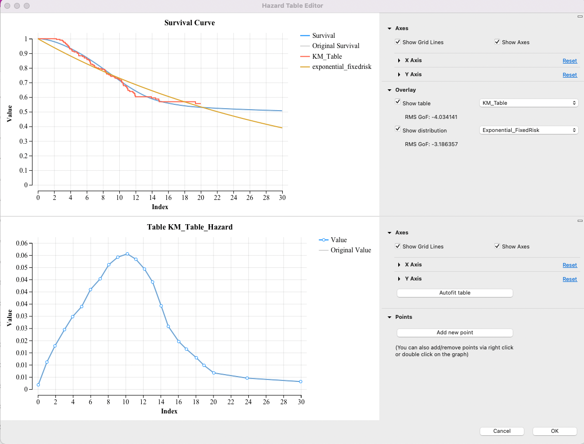
The figure below is the Hazard Function Editor showing the Survival Curve at the top generated from the Hazard Table below. On the right hand side of the Survival Curve we have selected to compare the Survival with both the Hazard Table and also the Exponential distribution in the model.

The formula for the Root Mean Square (RMS) formula for Goodness of Fit (RMS_GoF) is:

where:

• is the KM survival table function.

• is the Survival function computed from the hazard table or the distribution survival curve.

• is zero.

• is the end time of the KM survival table (the value in index column in the last row).

The RMS GoF is calculated as:

The use of the logarithm is “magnifying” the very small areas to make them more immediately recognized by observation.

Please note that this RMS_GoF is different than the goodness of fit metrics used in statistical regression, where maximum-likelihood methods are used based on the available data points to be approximated.

As with heuristic indicators of fit and parsimony (e.g. Akaike information criterion - AIC, Bayesian information criterion - BIC) one should not aim at “unreasonable” level of fit, which may actually be an overfit of the KM data (particularly for sparse data). The RMSGoF is simply a guide as to how close the KM and hazard derived curve are, and the user should use use better judgment as to how close is close enough.