38.5 Survival Functions
Each Survival Curve node (the branches from the PartSA node) requires a Survival Function to represent exit from the associated state to the next progression state. Typically, a Survival Function would be represented by one of the following.
-
A parametric distribution describing state membership.
-
A table describing state membership (Kaplan-Meier data).
-
A survival time function.
-
A hazard function.
38.5.1 Survival by Distribution
Frequently in PartSA models, survival analysis is performed to find a “best fit” distribution for event times for critical events like progression or death. This survival analysis would be perfomed outside of TreeAge Pro using statistical tools like SASS, STATA, R. TreeAge Pro supports many such distributions – Weibull, Exponential, Generalized Gamma, LogNormal, etc. These distributions represent time-to-event values for things like progression and death.
The time-to-event data is then transformed into survival functions using the function DistSurv. The DistSurv function returns the compliment of the cumulative distribution function (CDF) of the distribution. In essence, it returns the percentage of people who have not yet experienced the event at any time. With the distrbition referenced through the DistSurv function, you have your survival function.
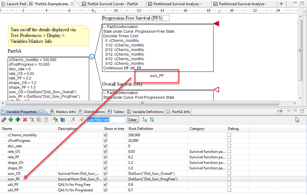
In the Healthcare Example model PartSA-Example.trex, there are two Weibull distributions. Each has its own scale and shape parameters.
-
Dist_Surv_ProgFree – describes state membership in the PFS state relative to the PPS state
-
Dist_Surv_Overall – describes state membership in the PPS state relative to the implicit dead state
The Survival functions using the DistSurv function are presented below.
-
PFS node: DistSurv(“Dist_Surv_ProgFree”)
-
OS node: DistSurv(“Dist_Surv_Overall”)
The DistSurv function has an implicit second argument referring to time.
The second argument has a default value of _time, which represents continuous time in the model. Therefore, DistSurv("Dist_Surv_ProgFree") is equivalent to DistSurv("Dist_Surv_ProgFree"; _time).
To incorporate distribution-based Survival into a model:
-
Create a distribution that describes survival against time. (See Distributions Chapter for details on creating a distribution). For example:
-
Create a Weibull distribution: Dist_Surv_ProgFree
-
The distribution parameters, as per the Example, are: rate_PF and shape_PF
-
-
Create a variable to reference the distribution/DistSurv function. In the example model this is: surv_PF = DistSurv("Dist_Surv_ProgFree")
-
Click below the Survival Curve node and enter the Survival Function, surv_PF.
Other forms of the DistSurv Function:
If your model time unit were annual, but your distribution described surivival in months, use the expression DistSurv("YourDist_Monthly"; _time*12).
For the opposite conversion of an annual distribution to a monthly model time unit, use the expression DistSurv("YourDist_Annual"; _time/12).
You can also calculate survival at a specific time with an expression like DistSurv("YourDist"; 5).
Additional options for the DistSurv function are specified in the Distribution Functions section of Help.
What does DistSurv calculate?
DistSurv("Dist_Name"; _time) returns the complement of the cumulative probability that an event has occurred at any given time. If a distribution represents progression, then DistSurv returns the probability that the progression has not yet occurred.
DistSurv("DistributionName") = 1 - DistProb("DistributionName";_time)
Using DistSurv with LogNormal or LogLogistic distributions
If the survival function uses a LogNormal or a LogLogistic distribution, this can produce an error when using DistSurv because Log(0) is undefined.
Instead of using DistSurv("distname"; _time) for Log Normal or LogLogistic distributions, use the following:
-
DistSurv("distname"; max(_time; 1e-12) )
The use of max(_time; 1e-12) will ensure 0 is never returned, and instead a very small number is used.
Note that some distributions (i.e., LogLogistic) are undefined at _time 0 in the context of PartSA models. You can set the minimum time to 0.0001 in such a distribution to allow for full survival for the small time interval between 0 and 0.0001 where the survival distribution is undefined.
38.5.2 Survival by Kaplan-Meier Table
Survival data is often recorded (and available) as a Kaplan-Meier table of data with the proportion of patients in a state at several times. This data can be used directly in the model.
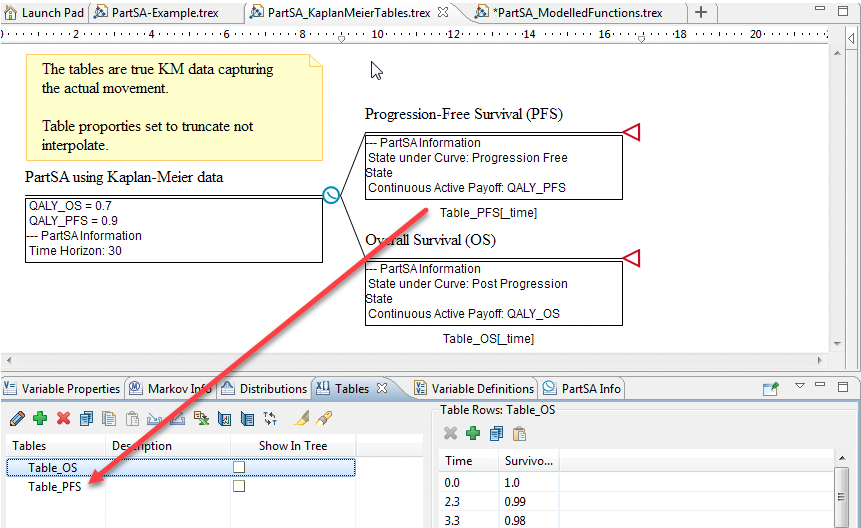
Using the Partitioned Survival Analysis Example Model, PartSA_KaplanMeierTables.trex, we represent the Survival Functions using Kaplan Meier data. The model structure is the same as in Example model described in the previous sections, with a PartSA node and two Survival Curve nodes representing PFS and OS curves.
Open the Tables View to examine the tables of Kaplan Meier data for PFS and OS. The data in the Table_PFS table shows the time in the first column (Index) and the proportion of the cohort that remains progression-free in the second column. The Table_OS table includes time in the first column and overall survival in the second. For example, in the Overall Survival State there is 1.0 (or 100%) of the cohort in the state at time 0. Later, at time 3.3 there is 98% (or 0.98) of the cohort in that health state.
The table properties are set with the lookup method truncate (as opposed to interpolate). This will generate a step-like survival curve beween values in the table. The lookup methoe interpolate would smooth out the data by interpolating in between time values provided.
To incorporate Kaplan Meier-based Survival functions into a model:
-
Create a table of Kaplan-Meier data: the first (Index) column is the times and the second column the proportion of the cohort in the given state. This information can be copied and pasted from Excel.
-
The Survival Functions simply look up the survival data at any given time directly from the table.
-
PFS node: Table_PFS[_time]
-
OS node: Table_OS[_time]
-
With the table lookup referencing the keyword _time, the table data is read and applied as time within the model passes.
If the table instead showed the percentage that had left the state (say percent dead for overall survival), then the Survival Function would be 1 - Table_Dead[_time].
38.5.3 Survival by Time Formula
You can also create an explicit survival function which calculates survival based on the current time value via the keyword _time. You could use this if your model's survival function does not fit a typical parametric distribution, but it can be represented by a formula. We call this a Survival Time Function, which describes exit from a health state at a given time.
To incorporate Survival Functions as a Survival Time Function:
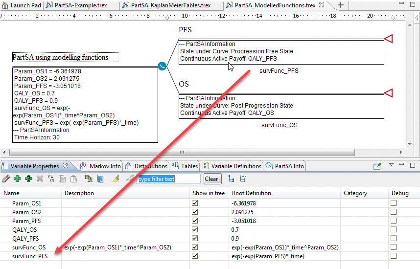
Using the Partitioned Survival Analysis Example Model, PartSA_SurvivalTimeFunction.trex, we can see an example of when the proportion of the cohort in each state is described using a function.
-
Create a variable in the Variables View that describes the time functions for each of the states in the model. In this example, examine the variables:
-
survFunc_PFS
-
survFunc_OS
-
These are both functions of time and other parameters. The functions describe the proportion of the cohort in each state with time (exactly what we need for our Survival Curve nodes).
-
-
Enter these functions directly under the appropriate branches of the PartSA nodes:
-
PFS node: survFunc_PFS
-
OS node: survFunc_OS
-
38.5.4 Survival by Hazard Function
Survival can also be defined by a Hazard function. The hazards might be defined by a Hazard table that describes the changing hazards over time. Refer to the help section Editing and Extending a Hazard Table for details on editing a hazard table and the resulting impact on survival.
The Healthcare Example model Hazards-CDC-PartSA.trex contains a single survival curve node for overall survival. It is defined by a hazard function that pulls hazard data from a hazard table derived from CDC data.
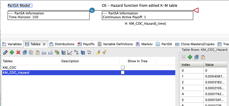
The hazards from the table are applied continuously with the hazard changing as time passes, resulting in an overall survival curve that matches the CDC survival data from which the hazard table was derived.
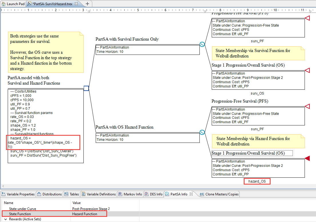
To compare survival and hazard functions, the Partitioned Survival Analysis Example Model, PartSA-SurvVsHazard.trex includes two strategies that are nearly identical.
This model has equivalent strategies, designed to allow the comparision of the model outputs using different forms of the same Survival Function.
-
The top strategy uses the Weibull distribution directly in calculating the Survival Function for the Overall Survival. Specifically, the survival function for Post-Progression is: surv_OS = DistSurv("Dist_Surv_Overall")
-
The bottom strategy uses a Hazard Function based on the Weibull distribution hazard function for Overall Survival. Specifically, the survival function for Post-Progression is: hazard_OS = rate_OS*shape_OS*(_time^(shape_OS + 1)).
-
Both functions use the same Weibull distribution parameters, defined by variables rate_OS and shape_OS.
To incorporate Survival Functions as Hazard Functions:
-
Create a variable which describes the Hazard Function. For example:
-
The parameters, as per the Example, are: rate_OS and shape_OS.
-
The variable defining the Hazard function is: hazard_OS = rate_OS*shape_OS*(_time^(shape_OS - 1))
-
-
Click below the Survival Curve node and enter the Survival Function, hazard_OS.
-
Select the Survival Curve node, open the PartSA View. In the row where it says State Function, select the option: Hazard Function.
In this example model, the variable hazard_OS contains the Weibull hazard function formula. The model is designed so you can compare the use of the Weibull Distibution and the DistSurv function directly against the Weibull Hazard Function.
The ability to use hazard functions provides flexibility for use of other parameters within hazard functions to account for individual characteristics and/or treatment effects (e.g., Cox Regression models).
38.5.5 Survival by Kaplan-Meier and Distribution
Survival data is often recorded (and available) as a Kaplan-Meier table of data with the proportion of patients in a state given at different times. This data can be used directly in a Partitoned Survial Analysis model, as detailed in the section above.
However, after a certain period of time, it maybe necessary to use an estimate for the progression. A distribution is usually defined to represent the data going forward in time. This section defines how to combine both Kaplan-Meier and Distributions in a model.
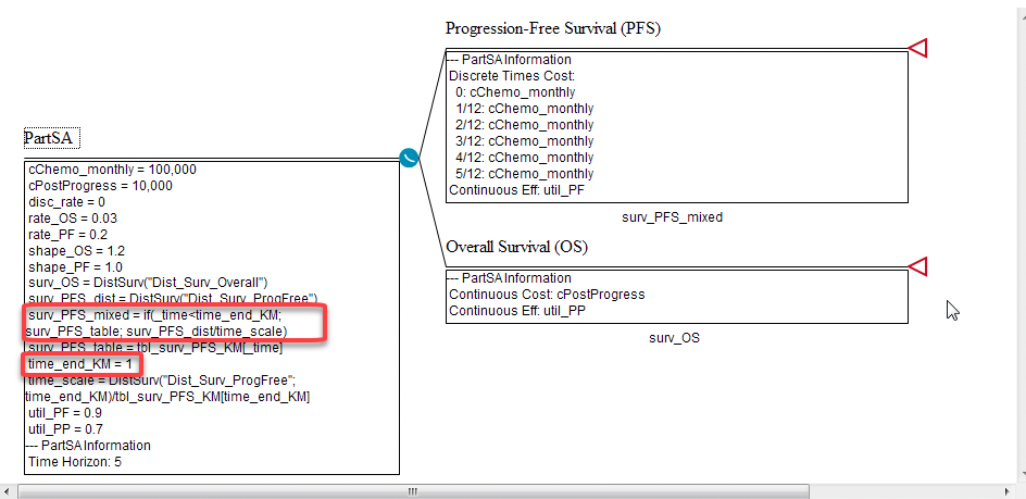
The Partitioned Survival Analysis Example Model, PartSA-KaplanMeier_and_Distribution.trex includes a function which combines both of these.
To incorporate Survival as functions of Kaplan-Meier tables and Distributions:
-
Create a table of Kaplan-Meier data: the first (Index) column is the times and the second column the proportion of the cohort in the given state. This information can be copied and pasted from Excel. In this model, the table tbl_surv_PFS_KM is for the PFS state and referenced by the variable:
-
surv_PFS_table = tbl_surv_PFS_KM[_time]
-
-
Create a distribution that describes survival against time. (See Distributions Chapter for details on creating a distribution). For example:
-
Dist_Surv_ProgFree – describes state membership in the PFS state relative to the PPS state
-
It is a Weibull distribution with parameters: shape_PF and rate_PF
-
-
Create a variable to reference the distribution. In the example model this is: surv_PFS_dist = DistSurv("Dist_Surv_ProgFree")
-
Create a variable to define the time at which you want Survival to switch from Kaplan Meier data to the distribution. In this example: time_end_KM = 1
-
Create a time dependent variable which will get the Survival Function at the correct time:
-
surv_PFS_mixed = if( _time < time_end_KM; surv_PFS_table; surv_PFS_dist/time_scale)
-
The variable time_scale is used to normalise the values between the last Kaplan-Meier table entry used at _time = time_end_KM and the start of the first value from surv_PFS_dist. This eliminates discountinuity between the two calculations at the switch time.
-
-
Click below the Survival Curve node for PFS and enter the Survival Function, surv_PFS_mixed.
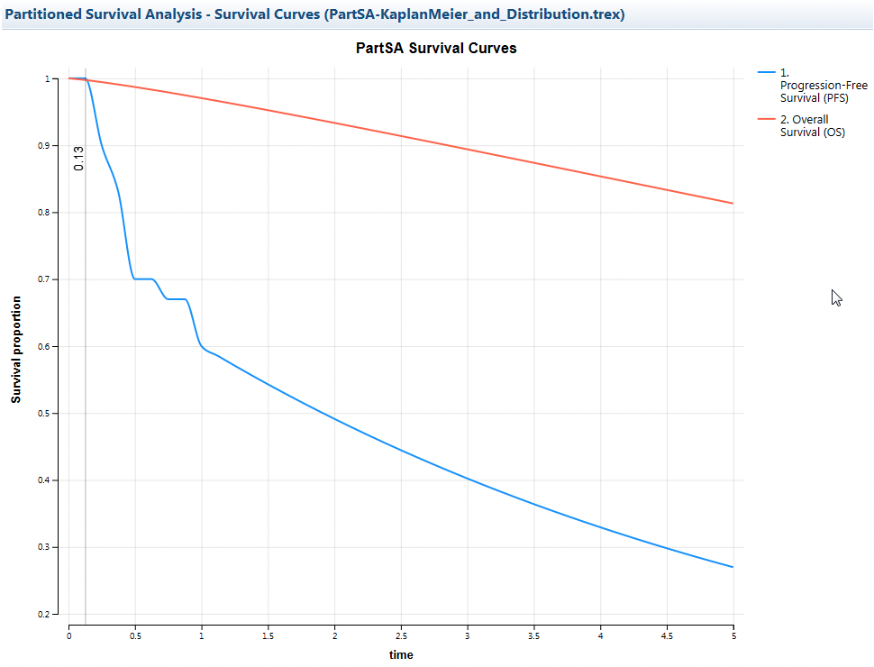
The Survival Curve for this model will be a combination of both a step-wise function and the smoother curve from the distribution.
38.5.6 Survival for Mixture Cure Models and Mixture Models
Mixture Cure and Mixture models use a combination of survival functions to represent survival for a single heath state.
Mixture Cure Models
In a Mixture Cure model, it is presumed that a fraction of the cohort in the Post-Progression State (PPS) are cured and only subject to risk of death by background mortality. The PPS survival function combines calculations from both background mortality and excess risk from the disease.
The elements required for Mixture Cure models is shown below.
-
S_mixed(t) = S_background(t) * (pct_cured + (1-pct_cured) * S_disease_excess(t))
-
S_mixed(t) is mixed overall survival
-
S_background(t) is survival derived from background mortality
-
S_disease_excess(t) is survival derived from the excess risk of death from disease
-
pct_cured is the percent of cohort that is cured
In essence, the formula breaks the cohort state membership into two groups - cured and uncured - and combines survival for those groups into a single survival function.
The Partitioned Survival Analysis Example Model, PartSA-MixtureCure.trex demonstrates this technique.
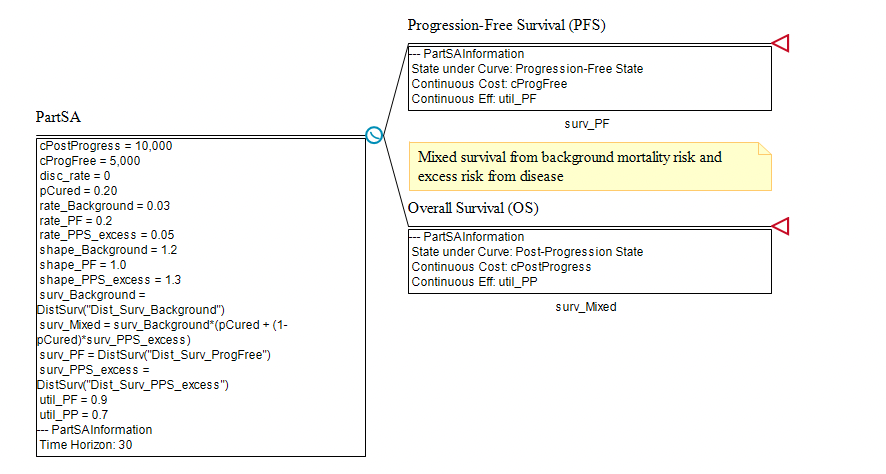
Note the following inputs of the model representing the list of required elements needed for a Mixture Cure model.
-
surv_Mixed = surv_Background*(pCured + (1-pCured)*surv_PPS_excess)
-
surv_Background = DistSurv("Dist_Surv_Background")
-
surv_PPS_excess = DistSurv("Dist_Surv_PPS_excess")
-
pCured = 0.20
The mixed survival function surv_Mixed is then placed beneath the Overall Survival node. Note that if you increase the parameter pCured, the cohort will survive longer.
! Be careful with Mixture Cure models !
-
They assume that cured people are no longer subject to disease risk.
-
You need to isolate disease risk from background mortality.
Mixture Models
In a Mixture model, it is presumed that the cohort in the Post-Progression State (PPS) is subject to background mortality risk from disease. The PPS state is also broken into two subgroups with different excess risk from disease.
The elements required for Mixture models is shown below.
-
S_mixed(t) = S_background(t) * (pct_mix1*S_disease_excess1(t) + (1-pct_mix1)*S_disease_excess2(t))
-
S_mixed(t) is mixed overall survival
-
S_background(t) is survival derived from background mortality
-
S_disease_excess1(t) is survival derived from the excess risk of death from disease for subgroup 1
-
S_disease_excess2(t) is survival derived from the excess risk of death from disease for subgroup 2
-
pct_mix1 is the percent of cohort that is in subgroup 1
In essence, the formula breaks the cohort state membership into two subgroups that face different disease-related risk. These elements are applied in the model below.
The Partitioned Survival Analysis Example Model, PartSA-Mixture.trex demonstrates this technique.
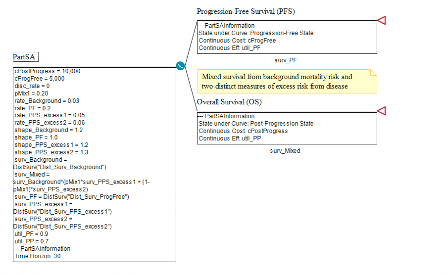
Note the following inputs of the model representing the list of required elements needed for a Mixture model.
-
surv_Mixed = surv_Background*(pMix1*surv_PPS_excess1 + (1-pMix1)*surv_PPS_excess2)
-
surv_Background = DistSurv("Dist_Surv_Background")
-
surv_PPS_excess1 = DistSurv("Dist_Surv_PPS_excess1")
-
surv_PPS_excess2 = DistSurv("Dist_Surv_PPS_excess2")
-
pMix1 = 0.20
The mixed survival function surv_Mixed is then placed beneath the Overall Survival node.
In this example, the survival for those in subgroup 1 is greater than the survival for those in subgroup 2. In the model, if you increase the parameter pMix1, the cohort will survive longer because the risk for subgroup 2 is greater (higher rate) than the risk for subgroup 1 (i.e., therefore increasing the proportion of the cohort - subgroup 1 - who live longer).