Partitioned Survival Analysis: An Example

38.1 Partitioned Survival Analysis: An Example

This section will examine the Partitioned Survival Analysis Example Model PartSA-Example.trex which follows cancer progression. We will look at the basic elements of this PartSA model in this section. Further details including implementation instructions are provided in subsequent sections of this chapter.

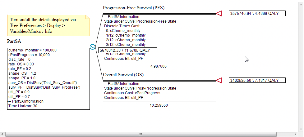
In PartSA models, disease progression is represented by a series of Survival Curve nodes, each of which has an underlying health state. Survival Curve nodes are ordered with the healthiest Survival Curve/state at the top and the sickest at the bottom, implying a top down progression through all states to an implicit Dead state following the bottom branch. The figure below shows the PartSA-Example.trex with PartSA node and general descriptions for each Survival Curve node

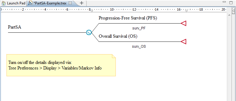
In this example model, there are three nodes:

A PartSA node representing the start of the PartSA model structure;
A Survival Curve node representing Progression-Free Survival (PFS); and
A Survival Curve node representing Overall Survival (OS).

The Dead state is implicit, so it is not included in the model structure. If there were more non-dead states, you would add more Survival Curve nodes.

Each Survival Curve node requires the following information:

Health State: the name of the health state whose exit is defined by the Survival Curve. For example: Progression-Free State for the top branch.
Survival Function: the Survival Function defines how the cohort exits the state over time. For example the expression surv_PF describes exit from the Progression-Free State. This function would be derived from patients' times of progression.
State Rewards: define how costs and utility is accumulated based on state membership.

Entry of the information as above is described in the Enter Partitioned Survival Analysis Node Inputs and the Enter Survival Curve Node Inputs sections.

The Survival Function for Progression-Free Survival is defined by the variable: surv_PF. This variable function calculates exit from the Progression-Free Survival State based on an underlying Weibull distribution, Dist_Surv_ProgFree. We will discuss Survival Functions in detail in the Survival Functions section.

Based on the model's two Survival Functions, the PartSA model generates the following Survival Curve Graph.

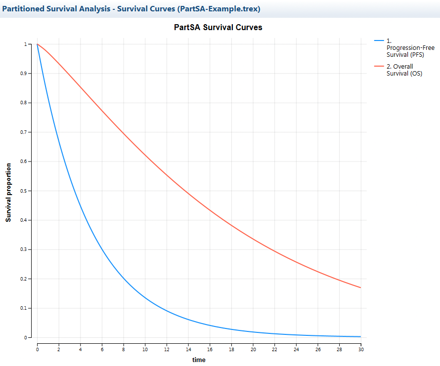
The PFS survival function represents the percentage of the cohort who have not yet progressed, derived from patient progression times. Patients who have not yet progressed can be considered to be in the Progression-Free state (PFS).

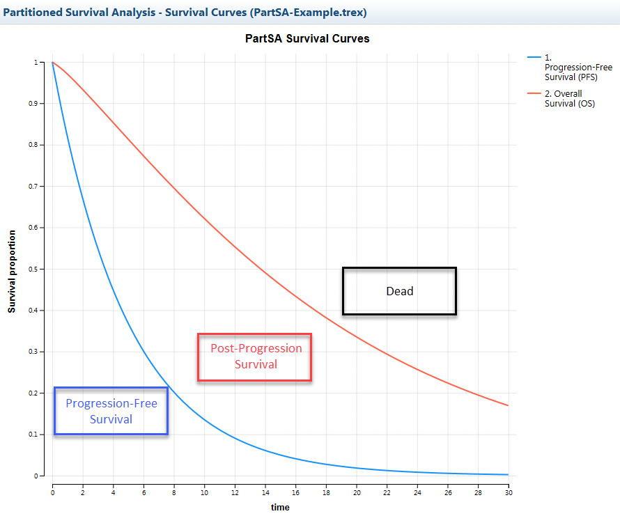
The OS survival function represents the percentage of the cohort who have not yet died, derived from patient death times. Patients who have not yet died can be considered alive. Therfore the people in the area between the PFS and OS curve can be considered to be in the Progression-Free state (PFS).

The health states are shown explicitly in the graph below.

With the Survival Curves in place to describe health state membership, we can now accumulate value – cost and effectiveness – based on state membership. Both cost and effectiveness are accumulated for the PFS and the PPS states.

In the PFS state, costs are accumulated at discrete times based on the percentage of the cohort in the associated PFS state. Our time unit is annual, and Chemotherapy is given once per month for 6 months – at times 0, 1/12, 2/12… 5/12. Utility is accumulated continuously from state membership based on the area under the curve. In the PPS state, both cost and utility are accumulated continuously based on state membership.

If you run Analysis > Roll Back on the model, you will see the total cost and effectiveness accumulated over the time horizon: $613,870.53 and 6.5596 QALYs. In a decision model, these values would be used in Cost-Effectiveness Analysis to compare this PartSA model to another strategy. Turn off Roll Back when you are done.

Select the PartSA node, and choose Analysis > Partitioned Survival Analysis > State Report to see details on how each health state contributed to the overall calculations shown in Roll Back. The report also provides the area under the curve for each state, including the implicit Dead state, which represents the total time spent in each state.

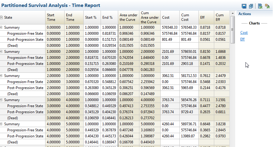
To see the total time horizon broken down into shorter time periods, select the PartSA node, and choose Analysis > Partitioned Survival Analysis > Time Report to see details on how each health state contributed to the overall calculations (State%, Cost and Effectiveness) broken down into discrete time periods.