41.1 Deterministic Sensitivity Analysis and Microsimulation
With microsimulation models, it is possible to run deterministic sensitivity analysis and Tornado Diagrams.
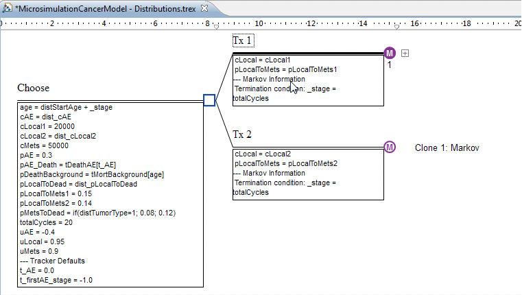
Consider the Health Care tutorial example model, MicrosimulationCancerModel - Distributions.trex.
1-Way Sensitivity Analysis and Microsimulation
This model requires Microsimulation because it uses individual trial-level distributions and trackers. However, we also want to run one-way sensitivity analysis on the variable cLocal2.
To run one-way sensitivity analysis:
-
Select the root (decision) node.
-
Choose Analysis > Sensitivity Analysis > 1 Way.
-
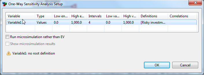
Choose the variable cLocal2 and enter the low, high and interval values as seen below.
-
Select the option "Run microsimulation rather than EV". (The Legacy option is below but this is a slower way of running 1-way and Microsimulation)
-
Click OK.

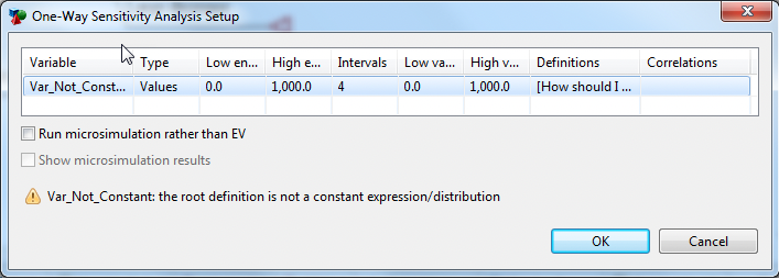
You will receive a warning if the variable you have selected for Sensitivity Analysis is not a variable defined at the root node and a variable defined as a number or as a distribution. You will receive a warning if you select a variable that does not appear to be a parameter. See figures below.
Warning if the variable selected for 1-Way Sensitivity Analysis is not a variable defined at the root node:
Warning if the variable selected for 1-Way Sensitivity Analysis is not defined as a constant or a distribution:
We selected to run Microsimulation rather than Expected Value calculations for this model. Therefore, the Monte Carlo simulation dialog is then presented to enter the number of trials, as below.
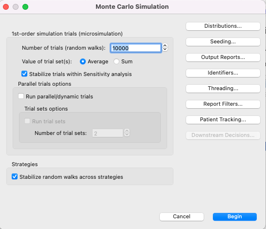
The check box "Stabilize trials within Sensitivity analysis" is automatically selected. This ensures the same sequence of random numbers is used for patients passing through the model.
All the options available in this dialog are described in a previous section when running Patient Level Simulation.
Based on the sensitivity analysis options, the analysis will consider values of $20K, $21K, $22K, $23K and $24K for variable cLocal2. In a regular sensitivity analysis, expected values would be generated for each variable value using Markov Cohort Analysis. Because this is a Microsimulation model within the sensitivity analysis, five separate microsimulations are executed, one for each variable value.
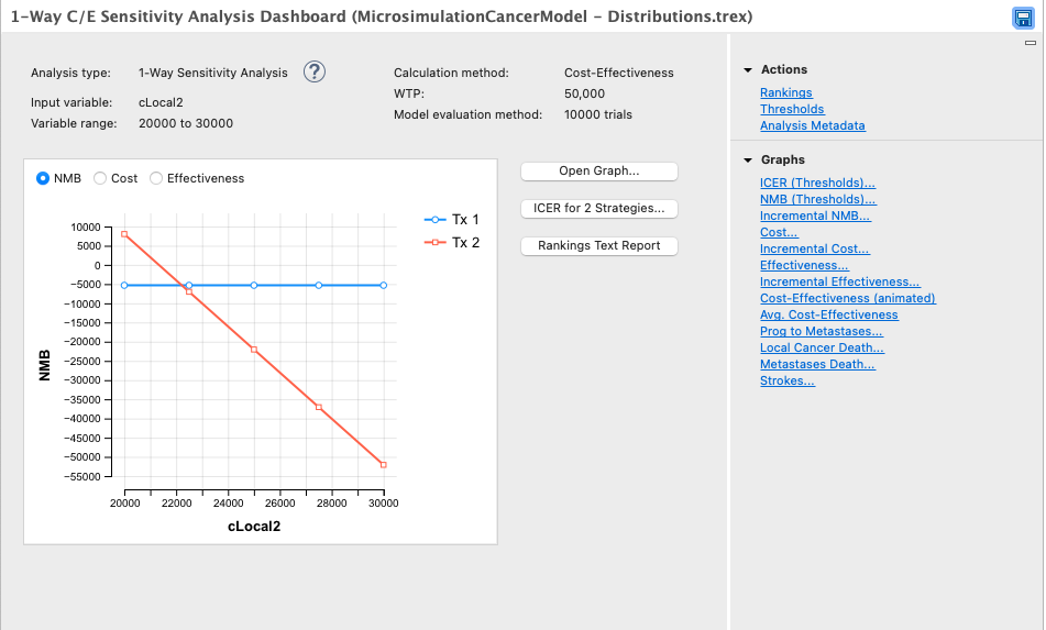
The Sensitivity Analysis Dashboard presents the outcomes of all five sets of Microsimulation results which are used to generate the five sets of sensitivity analysis outputs. The mean values from each set of Microsimulation results are used for the sensitivity analysis EV results. These mean values for NMB, Cost and Effectiveness are plotted on the graph seen in the Dashboard.
The graph in the dashboard for the Net Benefits (CE Thresholds) graph (with WTP = 50,000) shows there is a threshold in the range at cLocal2 = 22,218, a strategy change from one treatment to another. The details of this can be seen better by selecting the link "Open Graph..." to generate the usual NMB graph (as described in Outputs of One-Way Sensitivity Analysis CE models
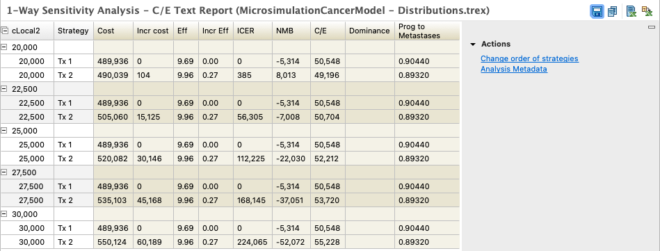
Other standard sensitivity analysis outputs as described in earlier sections can be seen selecting the appropriate links. Selecting the Rankings Text Report provides the image below which is standard 1-way Sensitivity Analysis output.
Tornado Diagram with Microsimulation
This model requires Microsimulation because it uses individual trial-level distributions and trackers. However, we also want to generate a Tornado diagram for a number of on the variables.
To run a Tornado Diagram:
-
Select the root (decision) node.
-
Choose Analysis > Sensitivity Analysis > 1 Way.
-
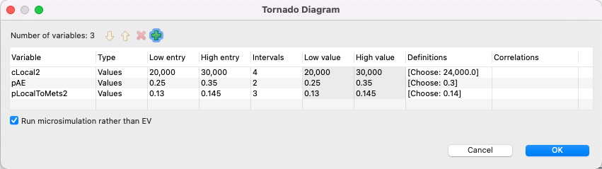
Choose the variables to include with the low, high and interval values as seen below.
-
Select the option "Run microsimulation rather than EV".
-
NOTE: For every combination of variables, the model will need run a microsimulation so consider this in terms of the time it takes to evaluate the model.
-
Click OK.
Be careful not to select variables that are formulas, rather than numeric parameters defined at the root node. A warning will alert you to this issue if you have selected such a variable (as demonstrated in the 1-way sensitivity section above).
When we run Microsimulation, the Monte Carlo simulation dialog is then presented to enter the number of trials, as before. Note the "Stabilize trials within Sensitivity Analysis" option is selected to ensure there is consistency among all trial sets.
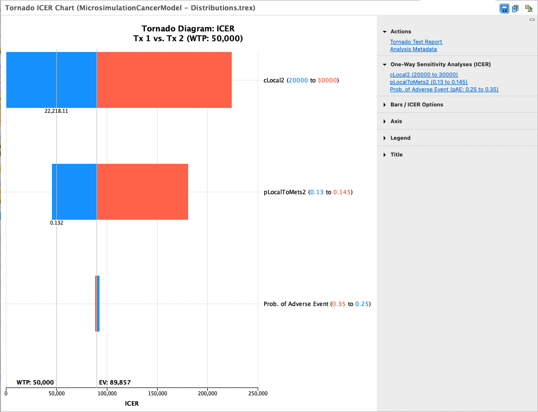
Once the Tornado Diagram opens, all the options available in this dialog are described in the Tornado diagrams outputs for CE models section. The ICER tornado is show below.
2-Way and 3-Way Sensitivity Analysis and Microsimulation
This model requires Microsimulation because it uses individual trial-level distributions and trackers. However, we also want to run 2- or 3-way sensitivity analysis on some variables.
To run 2-way or 3-way sensitivity analysis:
-
Select the root (decision) node.
-
Choose Analysis > Sensitivity Analysis > 2 Way or 3 Way.
-
Choose the variables to include, with appropriate ranges. (You can use the defalut in the example model).
-
Set the vaue of either NMB or NHB as the calculation type. This provides the value against which we can compare the strategies.
-
Select the option "Run microsimulation rather than EV".
-
NOTE: For every combination of variables, the model will need run a microsimulation so consider this in terms of the time it takes to evaluate the model.
-
Click OK.
For 2-way sensitivity analysis, the resulting graph is shown below. It identifies which strategy is optimal in regions of values of the variables; thresholds are simply the border between two regions.
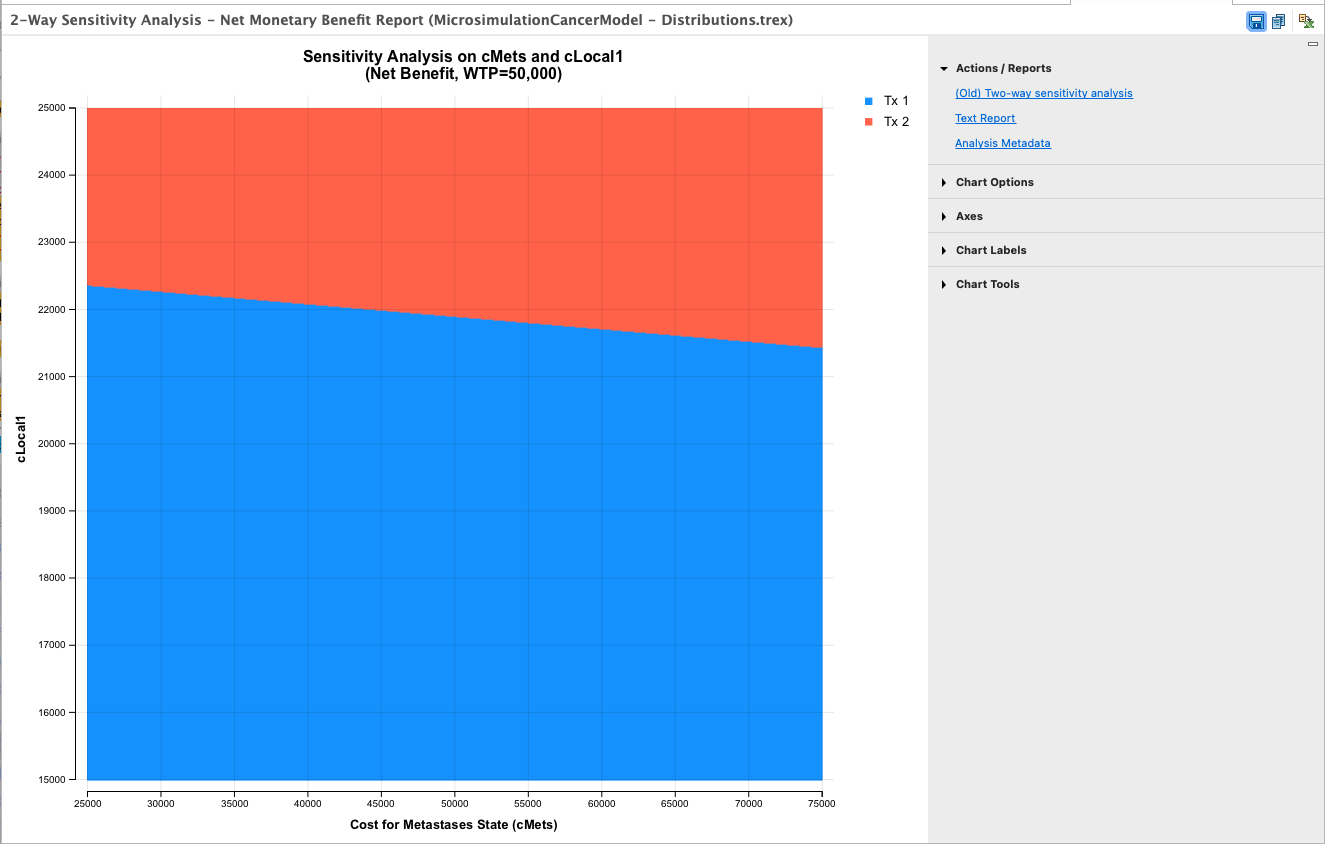
Find out more about 2-way sensitivity analysis in the section: 2-way CE sensitivity analysis thresholds using Net Benefits.
Three variables cannot be presented as clearly as in a two-dimensional graph. Therefore, the results of a three-way sensitivity analysis are presented as an animated two-way sensitivity analysis region graph. The third variable is represented not with its own axis, but rather using a series of two-way graphs — if four intervals are specified for the third variable, then five graphs will be created, and shown in series.
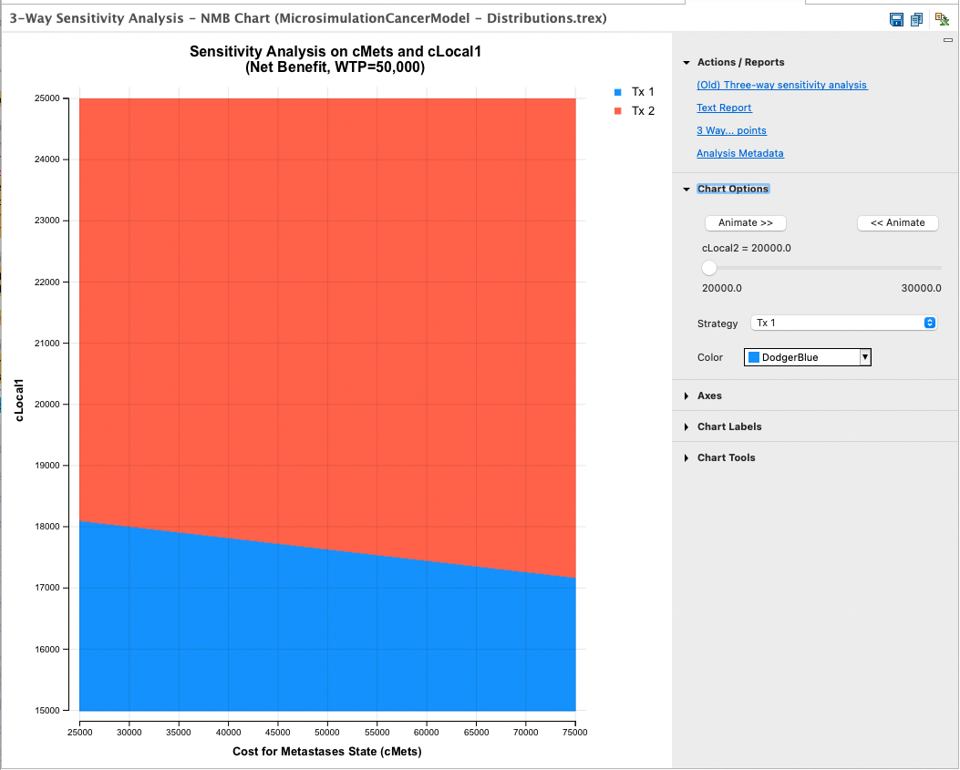
Under Chart Options (on the right-hand side) use the Animate button or the scroll bar to cause the third variable (cLocal2) to cycle through its range. The successive frames of the three-way analysis shows how the two-way region/optimality graph for the first two variables is affected by varying the value of the third variable.
Find out more about 3-way sensitivity analysis in the 3-way CE sensitivity analysis thresholds using Net Benefits section.